phasr is a python package able to calculate scattering phase shifts for arbitrary radial potentials and calculate (elastic) electron nucleus scattering cross sections based on it.
In combination with a fitting routine it can be used to fit elastic electron nucleus scattering data to extract charge density parameterizations. It is also possible to increase the precision sufficiently to quantitatively resolve parity violating electron scattering.
Since Version 0.5.0 a module with fitting routines for the purpose of extracting charge distributions from elastic electron nucleus scattering is also part of the package.
Version 0.5.3 : Fix some bugs.
Version 0.5.2 : Fix some bugs.
Version 0.5.1 : Add cross_section_fitter module.
Version 0.4.0 : Add left-right asymmetry.
Version 0.3.2 : Extend docs.
Version 0.3.1 : Add access to reference parameterizations.
Version 0.3.0 : Add overlap integrals.
Version 0.2.2 : Fix some dependencies.
Version 0.2.1 : First PyPI Release.
Version 0.2.0 : Basic features implemented.
Version 0.1.4 : Build dirac_solvers module.
Version 0.1.3 : Build nuclei module.
Version 0.1.2 : Build skeleton.
Version 0.1.0 : First init. Empty.
This package was developed with the goal of extracting charge density parameterizations based on (elastic) electron nucleus scattering cross section data while properly accounting for Coulomb corrections using the so called phase shift model. While this procedure is known since the 60s, the documentation and availability of programs used back then, are very limited and hardly accessible. Furthermore, for a majority of nuclei the extractions of model-independent parameterizations of their charge densities have not been updated since the 80s and do not provide any uncertainty estimates. Since these also applied to the nuclei we were interested in, we build such a framework in Python, which calculates elastic electron nucleus scattering cross sections based on input charge densities using the phase shift model, from which this package evolved. With such a more modern implementation and programming language, the calculations can become faster, broader accessible, easier to understand and easier to incorporate into existing programs. The code leading up to this package has already been used successfully in the papers [Noël, Hoferichter - 2024] and [Heinz, Hoferichter, Miyagi, Noël, Schwenk - 2024] to calculate and extract charge distributions for nuclei of interest to \( \mu \to e \) conversion, a beyond the Standard Model process of interest in particle physics as well as parity violating electron scattering. The package has been successfully employed for nuclei reaching from \(^{27}\)Al to \(^{208}\)Pb .
This program is built with/for python 3.
It requires the following packages to operate properly:
numpy
scipy
mpmath
To install and use the program please follow the following steps for setup. We assume you already have a working python environment setup on your machine.
The package is listed on PyPI, which is why it can be easily installed via:
pip install phasr You can import the python package the same way as every other package, i.e.:
import phasr as phr nucleus_Al27 = phr.nucleus(name='Al27',Z=13,A=27,rc=5)
mmu = phr.masses.mmu
boundstates_Al27 = phr.boundstates(nucleus_Al27,kappa=-1,lepton_mass=mmu)
print('E_1s=',boundstates_Al27.energy_levels[0],'MeV') phr throughout this manual.
The code is structured into two main modules.
The nuclei module is home of the nucleus class and manages all the relevant properties of a nucleus/isotope that is considered and calculates other properties based on the information it has available (e.g. the electric field from the charge density).
The dirac_solvers module is home of the boundstates and continuumstates classes and manages solving the Dirac equation for a given nucleus based on its nucleus potential and returns the desired consequential quantities like for example electron wave functions, phase shifts or the crosssection.
In all applicational scenarios one will first construct a nucleus object, which is then be used to construct a boundstates or continuumstates object. For calculating elastic scattering crosssections we supply the function crosssection_lepton_nucleus_scattering,
which can be used to directly calculate the crosssection using the energy, the angle and a nucleus object.
nucleus class To get a nucleus parameterization, use the nucleus class to construct a nucleus object.
A nucleus object requires a few minimum parameters (e.g. a name, a charge \(Z\) and a nucleon number \(A\)) and and has a lot of optional parameters (e.g. some parameters for a specific parameterization).
Based on the parameters supplied the class decides what kind of nucleus it is supposed to construct. You can check what parameterization was choosen based on the attribute nucleus_type
phr.nucleus(name,Z,A,m=None,**args) | nucleus_type | Parameters / **args |
|---|---|
| 'coulomb' | None |
| 'fourier-bessel' | ai (1d-array): Array of parameters \(a_i\) in fm\(^{-3}\). \(N\) given by length of a.
R (float): Cutoff radius R in fm. |
| 'oszillator-basis' | Ci_dict (dict): dictionary of 1d-arrays \(C_i\), with multipole names as keys (see below). |
| 'fermi' | c (float): \(c\) parameter in fm for Fermi parameterization.
z (float): \(z\) parameter in fm for Fermi parameterization. w (float,optional): \(w\) parameter for Fermi parameterization (default: w=0). |
| 'gauss' | b (float): \(b\) parameter in fm for Gauss parameterization. |
| 'uniform' | rc (float): \(r_c\) parameter in fm for Uniform parameterization. |
| 'numerical' | see below |
nucleus object can have the following attributes (if the prerequisites are met), that you might want to access
| Parameters/**args | |
|---|---|
| charge_density (callable,optional): | Function describing the charge density (see below). |
| form_factor (callable,optional): | Function describing the form factor (see below). |
| electric_field (callable,optional): | Function describing the electric field (see below). |
| electric_potential (callable,optional): | Function describing the electric potential (see below). |
| form_factor_dict (dict,optional): | Dictionary containing form factor functions for specific multipoles (keys are 'F'+multipole , see below). |
| density_dict (dict,optional): | Dictionary containing density functions for specific multipoles (keys are 'rho'+multipole , see below). |
| rrange (list,optional): | Sets range parameters for the beginning of the integration and highenergy continuation (in fm, default: [0.,20.,0.02]). |
| qrange (list,optional): | Sets range parameters for the beginning of the integration and highenergy continuation (in MeV, default: [0.,1000.,1.]). |
| renew (bool,optional): | Says if numerical calculations should be done from scratch (aka renewed) or recovered from file if existent (default: False). |
multipoles. Fch(q,L=0), Fw(q,L=0), Fmag(q,L=1), which make it possible to also access the form factors for higher \(L\) if the necessary multipoles were supplied.
dirac_solvers moduleThe dirac_solvers module has two main duties, covered by two classes.
The boundstates class calculates the boundstate solutions of a given nucleus by solving the Dirac equation in the presence of the nucleus potential, which includes finding the boundstate energy first.
The continuumstates class calculates the continuumstate solution for a given energy of a given nucleus by solving the Dirac equation in the presence of the nucleus potential.
Finally, there are some functions that make use of the boundstate and continuumstate solutions by calculating elastic electron nucleus scattering crosssections and overlap integrals for \(\mu \to e\) conversion.
The boundstate and continuumstate wavefunctions are both parameterized according to
\[ \psi = \psi_\kappa^\mu(\vec{r})= \frac{1}{r} \Bigg(\begin{array}{c}
g_\kappa(r) \phi_\kappa^\mu(\hat{r}) \\ i f_\kappa(r) \phi_{-\kappa}^\mu(\hat{r}) \end{array} \Bigg), \]
separating off the angular degrees of freedom, which are the same for all radial symmetric potential. The \(\kappa\) label refers to the angular momentum quantum numbers and spin according to
\[j = |\kappa| - \frac{1}{2}; \quad l = \begin{cases} \kappa, & \quad \kappa > 0 \\ - \kappa - 1 , & \quad \kappa < 0 \end{cases}\]
The numerical calculations then provide descriptions for \(g_\kappa(r)\) and \(f_\kappa(r)\).
The boundstates class:
The boundstates class is used to calculate the boundstates for a given nucleus object, beginning from the ground state for the given partial wave.
First the energy for the boundstate is found by iteratively scanning for flips in the asymptotic behaviour of the wave functions, which indicate a boundstate in between, until a set precision is reached.
For this energy then the solution of the Dirac equation gives the dirac wavefunction for that state.
phr.boundstates(nucleus,kappa,lepton_mass,**args) phr.masses.me or muon mass phr.masses.mmu. needs to be non-zero.
scipy.integrate.solve_IVP). Default values are set by phr.default_boundstate_settings.
boundstates object has the following attributes, which you might want to access:
find_next_energy_level and solve_IVP_at_current_energy consecutively. Can be passed **args to change the solver_setting.
find_next_solution() was called enough times.
Example: Groundstate is wavefunction_g_1s12 (using \(\kappa=-1\))
find_next_solution() was called enough times.
Example: Groundstate is wavefunction_f_1s12 (using \(\kappa=-1\))
continuumstate class: phr.continuumstates(nucleus,kappa,energy,lepton_mass=0,**args) scipy.integrate.solve_IVP). Default values are set by phr.default_continuumstate_settings.
continuumstates object has the following attributes, which you might want to access:
solve_IVP() was called.
solve_IVP() was called.
solve_IVP().
crosssection_lepton_nucleus_scattering function: phr.crosssection_lepton_nucleus_scattering(energy,theta,nucleus,lepton_mass=0,recoil=True,subtractions=3,**args) optimise_crosssection_precision() (see below).
| Parameters/**args | |
|---|---|
| N_partial_waves (int,optional): | angular momenutum of the partial wave at which the series is terminated. (default: 100) |
| phase_difference_limit (float,optional): | limit at which (numerical) value for the phase_difference attribute of a continuumstates all following partial waves are considered indistinguishable to the coulomb solution. (default:0). |
| energy_norm (float,optional): | scaling factor for the units while solving the inital value problem to increase speed (default: \( \hbar c\) fm\(^{-1}\)) |
| method (str,optional): | method keyword passed to scipy.integrate.solve_IVP (default: 'DOP853' / as set in default_continuumstate_settings) |
| atol (float,optional): | atol keyword passed to scipy.integrate.solve_IVP (default: 1e-12 / as set in default_continuumstate_settings) |
| rtol (float,optional): | rtol keyword passed to scipy.integrate.solve_IVP (default: 1e-9 / as set in default_continuumstate_settings) |
crosssection_lepton_nucleus_scattering many times for the same energies and angles theta for similar nuclei (for example for a fit),
it makes sense to assess the necessary precision for the numerical calculation using optimise_crosssection_precision.
This functions can run a few minutes as it is scanning a large **args / parameter space, but can afterwards improve the runtime significantly.
Unfortunately the necessary precision is very dependent on how large the energy and angles are (larger energies and angles require significantly more precision and runtime),
which is why this is the best solution for a reasonable runtime. Of course you can always also try to finetune the parameters yourself, but note that the convergence might break down,
and that you should always check if the calculated crosssection is still reasonable.
phr.optimise_crosssection_precision(energy,theta,nucleus,lepton_mass=0,recoil=True,subtractions=3,crosssection_precision=1e-3,jump_forward_dist=1) crosssection_lepton_nucleus_scattering which are still consistent with crosssection calculations with the maximum precision up to a relative precision of the value of crosssection_precision.
left_right_asymmetry_lepton_nucleus_scattering function: crosssection_lepton_nucleus_scattering.
Requires a nucleus with a weak_potential, usually derived based on a weak_density. The nucleus for the charge interaction and the weak interaction may be choosen independenly.
left_right_asymmetry_lepton_nucleus_scattering(energy,theta,weak_nucleus,charge_nucleus=None,**args) crosssection_lepton_nucleus_scattering. atol and rtol are defaulted to 1e-13 / maximum precision
The time-optimal parameters for a given dataset can be accessed by calling optimise_left_right_asymmetry_precision() (see below).
left_right_asymmetry_lepton_nucleus_scattering works analogously to the optimise_crosssection_precision, with usually even longer runtimes.
phr.optimise_left_right_asymmetry_precision(energy,theta,nucleus,left_right_asymmetry_precision=1e-3,jump_forward_dist=1,N_processes=1) left_right_asymmetry_lepton_nucleus_scattering which are still consistent with left-right asymmetry calculations with the maximum precision up to a relative precision of the value of left_right_asymmetry_precision.
cross_section_fitter moduleThe cross_section_fitter module contains fitting routines to semi-automatically extract charge distrobutions including uncertainty bands from elestic electron nucleus scattering. For an example of how to employ these functions see below and the there discussed example notebook
ExamplesBasic.ipynb, which also repeats the examples shown here.
As of Version 0.5.0 another notebook ExamplesFit.ipynb with some auxilary files was added to show the usage of the fitting subroutines added in that update. See also the fit example shown below .
To calculate the scattering cross section base on a analytic charge distribution parametrisation, you first construct the nucleus object, which you then use to calculate the cross section. As an example, we use a Fourier Bessel parameterisation for \(^{48}\)Ti with \( R = 9.25\) fm and \[a_{1} = 0.03392 ~ \text{fm}^{-3}, ~ a_{2}=0.05913 ~ \text{fm}^{-3}, ~ a_{3}=0.01547 ~ \text{fm}^{-3}, ~ a_{4}=-0.02550 ~ \text{fm}^{-3}, \] \[a_{5}=-0.0152 ~ \text{fm}^{-3}, ~ a_{6}=0.0029 ~ \text{fm}^{-3}, ~ a_{7}=0.0037 ~ \text{fm}^{-3}, \] The nucleus is then constructed by
ai_48Ti=np.array([0.03392,0.05913,0.01547,-0.02550,-0.0152,0.0029,0.0037])
R_48Ti=9.25
nucleus_48Ti = phr.nucleus('48Ti_FB',Z=22,A=48,ai=ai_48Ti,R=R_48Ti)import matplotlib.pyplot as plt
energy=249.5
theta=np.arange(30,120,1e-1)
plt.plot(theta,phr.crosssection_lepton_nucleus_scattering(energy,theta*pi/180,nucleus_48Ti),label=r'$E=249.5~$MeV')
plt.yscale('log')
plt.title(r"Cross section $^{48}$Ti")
plt.xlabel(r"$\theta$ in deg")
plt.ylabel(r"$\frac{\operatorname{d}\sigma}{\operatorname{d}\Omega}$ in MeV$^{-2}$")
plt.legend()
plt.xlim(30,120)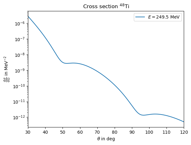
args=phr.optimise_crosssection_precision(energy,theta*pi/180,nucleus_48Ti,crosssection_precision=1e-2)import matplotlib.pyplot as plt
energy=249.5
theta=np.arange(30,120,1e-1)
plt.plot(theta,phr.crosssection_lepton_nucleus_scattering(energy,theta*pi/180,nucleus_48Ti,**args),label=r'$E=249.5~$MeV')
plt.yscale('log')
plt.title(r"Cross section $^{48}$Ti")
plt.xlabel(r"$\theta$ in deg")
plt.ylabel(r"$\frac{\operatorname{d}\sigma}{\operatorname{d}\Omega}$ in MeV$^{-2}$")
plt.legend()
plt.xlim(30,120)Calculating the scattering crosssection for a numerical charge density is for the most part identical to the analytical part. The only difference is that the nucleus object requires slighlty more preparation, as for example the nucleus potential needs to be calculated numerically. Let's construct the same nucleus as in the analytical case as a numerical nucleus. We do
ai_48Ti=np.array([0.03392,0.05913,0.01547,-0.02550,-0.0152,0.0029,0.0037])
R_48Ti=9.25
N_48Ti=len(ai_48Ti)
qi_48Ti = np.arange(1,N_48Ti+1)*np.pi/R_48Ti
def rho_48Ti(r): return phr.nuclei.parameterizations.fourier_bessel.charge_density_FB(r,ai_48Ti,R_48Ti,qi_48Ti)
nucleus_48Ti_num = phr.nucleus('48Ti_num',Z=22,A=48,charge_density=rho_48Ti)nucleus_48Ti_num.set_electric_field_from_charge_density()
nucleus_48Ti_num.set_electric_potential_from_electric_field()nucleus_48Ti_num.fill_gaps()energy=249.5
theta=np.arange(30,120,1e-1)
plt.plot(theta,phr.crosssection_lepton_nucleus_scattering(energy,theta*pi/180,nucleus_48Ti_num),label=r'$E=249.5~$MeV')
plt.yscale('log')
plt.title(r"Cross section $^{48}$Ti")
plt.xlabel(r"$\theta$ in deg")
plt.ylabel(r"$\frac{\operatorname{d}\sigma}{\operatorname{d}\Omega}$ in MeV$^{-2}$")
plt.legend()
plt.xlim(30,120)
plt.show()We consider a toy example for \({}^{208}\)Pb from a paper from [Horrowitz - 1998] . Here the weak density is considered to simply be the rescaled charge distribution with one additonal parameter to adjust the radius, according to \[ \rho^\lambda_\operatorname{w}(r) = \frac{Q_\operatorname{w}}{Z} \lambda^3 \rho_\operatorname{ch}(\lambda r) \] As the charge distribution he uses a 3pF parameterisation with \(c=6.4\), \(z=0.54\), \(w=0.32\) and for the rescaling \(\lambda=0.9502\). We may define a nucleus with these properties via
nucleus_Pb208 = phr.nucleus('Pb208_Hor98_095',Z=82,A=208,c=6.4,z=0.54,w=0.32)
def weak_density_model(r,lam,nucleus): return (nucleus.Qw/nucleus.Z)*lam**3*nucleus.charge_density(lam*r)
nucleus_Pb208.weak_density = partial(weak_density_model,lam=0.9502,nucleus=Pb208_test)
nucleus_Pb208.update_dependencies()
nucleus_Pb208.fill_gaps()update_dependencies() is run such that intermediate derivatives of weak_density like weak_potential are constructed.
Then fill_gaps() is run to calculate quantities than require explizit calculations like weak_radius. For the Fermi parameterizations this is also necessary to calculate related quantities to the charge_density like electric_potential. theta_deg=np.arange(1,50,1e-1)
E_MeV=850
A_PV_208Pb = phr.left_right_asymmetry_lepton_nucleus_scattering(E_MeV,theta_deg*pi/180,nucleus_Pb208,verbose=True)import matplotlib.pyplot as plt
plt.title(r'PVES $^{208}$Pb') #Horowitz 1998
plt.plot(theta_deg,A_PV_208Pb,label=r'$\lambda=0.9502$')
plt.ylim(0,4e-6)
plt.xlim(0,15)
plt.xlabel(r"$\theta$ in deg")
plt.ylabel(r"left-right asymmetry")
plt.legend()
plt.show()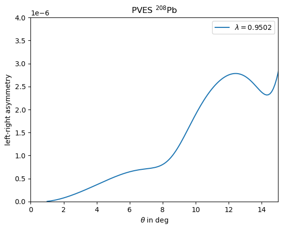
optimise_left_right_asymmetry_precision, which might take very long to run due to the increased runtime.
Using the the cross_section_fitter module to extract Fourier Bessel charge distributions from elastic electron nucleus scattering requires several steps, which require external supervison and decisions along the way.
We follow the fitting strategie as described in [Noël, Hoferichter - 2024] .
For the sake of this example we may seperate the fitting strategie into the following steps, which will be discussed in the following.
phr.import_dataset) phr.parallel_fitting_automatic) phr.cross_section_fitter.select_RN_based_on_property) phr.parallel_fitting_manual) phr.cross_section_fitter.split_based_on_asymptotic_and_p_val) phr.cross_section_fitter.promote_best_fit) ExamplesFit.ipynb notebook. Note that if you download the zip-archive all fits are already part of the archive, thus if you actually want to rerun any fits (which could be time intensive), you need to delete the respective files in the tmp folder.
Import and transformation of the experimental data
We consider having a file with rows of different data points where the columns contain inputs on the initial electron energy, the scattering angle and the measured elastic scattering crosssection ideally also containing columns for uncertainties.
We may then import and transform this data by running phr.import_dataset and answering the appearing questions, which will transform the data into the structure and units expected from the fitting routine.
For the sake of this example we may consider a dataset for \(^{40}\)Ar from [Ottermann et al. - 1982] , whos data we have written down in a file Ottermann1982_Ar40.txt.
We may load this dataset now with the intend of using it for a fit by calling (assuming that the file is in the same folder)
path_Ar40_Ot82 = "../Ottermann1982_Ar40.txt"
phr.import_dataset(path_Ar40_Ot82,"Ottermann1982",Z=18,A=40)What column (starting at 0) contains the central values for the energie? 0 In what units is the energy (MeV or GeV)? MeV What column (starting at 0) contains the central values for the angles? 1 In what units is the angle theta (deg or rad)? deg Does the file contain direct cross sections or relative measurements to a different nucleus? (answer with: direct or relative) direct What column (starting at 0) contains the central values for the cross section? 2 In what units is the cross section (fmsq, cmsq, mub, mb or invMeVsq)? fmsq Does the data distinguish between statistical and systematical uncertainties? (y or n) y What columns (starting at 0), if any, contain statistical uncertainties for the cross sections (separate by comma)? 3 Are the statistical uncertainties absolute values or relative to the central value? (answer with: absolute or relative) relative Are the relative statistical uncertainties in percent and thus need to divided by 100? (y or n) y What columns (starting at 0), if any, contain systematical uncertainties for the cross sections (separate by comma)? 4 Are the systematical uncertainties absolute values or relative to the central value? (answer with: absolute or relative) relative Are the relative systematical uncertainties in percent and thus need to divided by 100? (y or n) y Do you want to add a global relative statistical uncertainty w.r.t. the cross section as an (additional) uncertainty component? (For 3% insert 3, type 0 if you do not want to do so)? 0 Do you want to add a global relative systematical uncertainty w.r.t. the cross section as an (additional) uncertainty component? (For 3% insert 3, type 0 if you do not want to do so)? 0.8If you feel like you entered something wrong, you can always rerun this function, which will overwrite the existing prepared data. After this step the fitting routines can now identify this dataset by the unique label of "Ottermann1982" and the correct \(Z, A\). We can list all imported datasets for a given \(Z, A\) by calling
phr.cross_section_fitter.list_datasets(Z,A)
One may provide correlation matrices for statitistical and systematical uncertainties as additional arguments in the import_dataset function.
If these are not set, statistical uncertainties are considered completely uncorrelated and systematical uncertainties 100% correlated (considing they are in associaton with / dominated by normalisation uncertainties). phr.cross_section_fitter.import_barrett_moment, where the parameters and values are simply directly supplied (radii constrains can be considered as a special case of a barrett moment with \(k=2,\alpha=0\)).
Baseline fits
We may run baseline fits over a range of \(R,N\) to establish a minimum \(N\) for a given \(R\) range. We call for this phr.parallel_fitting_automatic. This function will derive how many \(N\) are covered by the exerimental data for a specific \(R\).
Then centered around this central value for \(N\) closeby values for \(N\) are choosen for the \(R,N\) pairs that should the fit should run for.
After the fits are run one should check if the lower borders of validity in \(R,N\) are sufficiently established or otherwise increase the range in \(R\) and/or \(N\).
Initial values for the fits are either taken from older fits with the same parameters, or from reference charge distributions from [De Vries et al. - 1987] (which can be accessed via phr.nuclei.load_reference_nucleus).
Before running all these fits it might make sense to establish the necessary precision for the cross section calculation to minimze runtime by running phr.optimise_crosssection_precision for the considered data points and a typical charge distribution as described above.
The call may then look like:
args_optimised =  {'method': 'DOP853', 'N_partial_waves': 25, 'atol': 1e-08, 'rtol': 1e-06, 'energy_norm': 0.001973269804, 'phase_difference_limit': 1e-06}
results_dict = phr.cross_section_fitter.fit_organizer.parallel_fitting_automatic(['Ottermann1982'],18,40,np.arange(4.00,8.75+0.25,0.25),redo_N=True,redo_aggressive=True,N_base_offset=1,N_base_span=3,cross_section_args=args_optimised)N_processes manually).
It makes sense to run this on a fast maschine with a lot of cores. It might still take between minutes to hours up to days to complete all fits, dependent on the used maschine and considered nucleus and datasets. Completed fits are saved and simply loaded if the function is run again with the same parameters and starting conditions.
The resulting results_dict is now a dictionary containing all fit results, from fitting against the 'Ottermann1982' dataset. Since we activated redo_N and redo_aggressive, after a first pass, individual fits were redone if any other fit result with the same \(R\) but smaller \(N\) had a better loss function, indicating that the fit did not find the best minimum yet.
Selection of \(R, N\)
We want to select a range of \(R, N\) with good statistics. We may generate 2d-arrays in \(R, N\) to study the statistical properties and if the studied range in \(R, N\) is sufficient.
We use the function phr.cross_section_fitter.generate_data_tables to prepare tables for different statistical properties. The pandas package is a good way to illustrate these 2d-arrays as tables in a jupyther notebook (you need to have this packege installed for this to work).
import pandas as pd
database_tables, Rs, Ns, hist = phr.cross_section_fitter.generate_data_tables(results_dict)
pd.DataFrame(database_tables['p_val'],index=Rs,columns=Ns)matplotlib package) via. Here you may choose to plot it like this
import matplotlib.pyplot as plt
plt.title('fit distribution')
plt.xlabel(r'$p_{val}$')
plt.plot([0.2,0.2],[0,42],color='red',linestyle='--')
plt.ylim(0,42)
plt.xlim(0,0.7)
plt.hist(hist['p_val'],10)
plt.show()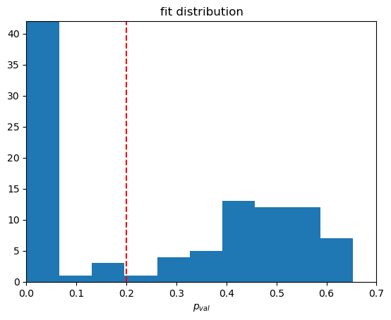
selected_RN_tuples = phr.cross_section_fitter.fit_organizer.select_RN_based_on_property(results_dict,'p_val',0.2) Final fits for our selection of \(R, N\)
We now perform the actual fits we want to use for our analysis. Here we only fit in the established window of values for \(R, N\) using the previous fit results as initial values. Here we also may now turn on additional constraints.
One additional contraint that we usually want to enable is a penalty on oscillations for large \(R\). A typical weight for this is monotonous_decrease_precision=0.04, in accordance with typical uncertainties on radii squared.
But if one has the computing resources one may play around with different values for this.
Other constraints are from Barrett moments (or radii squared as a special case), where we usually study fitting with or without them. These are included as an additional constraint in the same way as the datasets by listing keys of previously importet values.
A fit including barrett moments may look like
ini_settings = {'datasets':['Ottermann1982'],'datasets_barrett_moment':[],'monotonous_decrease_precision':np.inf}
results_dict_bar = phr.cross_section_fitter.fit_organizer.parallel_fitting_manual(['Ottermann1982'],18,40,selected_RN_tuples,redo_N=True,monotonous_decrease_precision=0.04,barrett_moment_keys=['Fricke1995_2p'],initialize_from=ini_settings,cross_section_args=args_optimised)
Selection of asymptotic confrom results
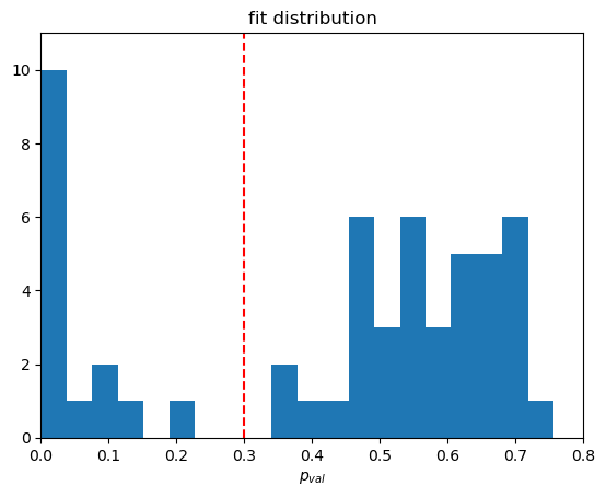
We can again study the statistical quantities of our fit results with the same tools as the baseline fits and find based on the histogram that a p value of 0.3 is a good cutoff.
We further veto all fits with bad asymptotic behaviour. For this we define three areas in \(q\) to match an upper limit for the asymptotic.
Ideally if the fits clearly contrains several minima in the form factor these regions should be seperated by the last clearly defined minimas, such that it matches onto the maximum values in the last two clearly defined areas.
We have a minimum falloff with \(q^{-4}\) which will jump in for our example case, since the data does not cover sufficent range in \(q\). We can study the resulting form factors and then choose
qs=[50,235,370,600]
results_dict_bar_sel, results_dict_bar_veto, veto_fct = phr.cross_section_fitter.fit_organizer.split_based_on_asymptotic_and_p_val(results_dict_bar,qs=qs,p_val_lim=0.3)results_dict_bar_sel dictionary now contains all fits we consider reasonable in describing the provided data without overparametrizating. The condition on the asymptotic should set an implicit upper limit on \(N\) for each \(R\). If this limit is not saturated yet, one might want to take a step back and extend the basefits to higher \(N\).
Select/Promote best fit and add systemetic uncertainty bands
One may now choose the best fit within the remaining sample usually by considering the fit with the best reduced \(\chi^2\). One way to select this could be to run
best_key_bar = None
best_p_val = 0
for key in results_dict_bar_sel:
p_val = results_dict_bar_sel[key]['p_val']
    if p_val > best_p_val:
        best_p_val = p_val
best_key_bar = keybest_key_bar, best_p_val contain the best p value and its corresponding dictionary key. We can now promote this fit to beeing the reference parameterization for this kind of nucleus, by calling
phr.cross_section_fitter.promote_best_fit(best_key_bar,results_dict_bar_sel)phr.cross_section_fitter.add_systematic_uncertainties to construct systematic uncertainty bands as an envelope around the selection of fits. Alternatively we can do this manually by calling
best_results_dict_bar = phr.cross_section_fitter.add_systematic_uncertainties(best_key_bar,results_dict_bar_sel)best_nuc_result = phr.nucleus('Ar40_FB_best_test',18,40,ai=best_results_dict_bar['ai'],R=best_results_dict_bar['R'])
best_cov_ai_model = best_results_dict_bar['cov_ai_model']
best_cov_ai_stat = best_results_dict_bar['cov_ai_stat'] * np.sqrt(best_results_dict_bar['redchisq'])
best_cov_ai_syst = best_results_dict_bar['cov_ai_syst']
r = np.arange(0,15,1e-2)
best_rho = best_nuc_result.charge_density(r)
plt.plot(r,best_rho,color='C0',zorder=2,label='best fit')
best_jac_rho = best_nuc_result.charge_density_jacobian(r)
best_drho_model = np.sqrt(np.einsum('ij,ik,kj->j',best_jac_rho,best_cov_ai_model,best_jac_rho))
best_drho_stat = np.sqrt(np.einsum('ij,ik,kj->j',best_jac_rho,best_cov_ai_stat,best_jac_rho))
best_drho_syst = np.sqrt(np.einsum('ij,ik,kj->j',best_jac_rho,best_cov_ai_syst,best_jac_rho))
plt.plot(r,best_rho+best_drho_stat,color='C0',linestyle=':',zorder=1,label='stat. error')
plt.plot(r,best_rho-best_drho_stat,color='C0',linestyle=':',zorder=1)
plt.plot(r,best_rho+best_drho_syst,color='C0',linestyle='--',zorder=1,label='syst. error')
plt.plot(r,best_rho-best_drho_syst,color='C0',linestyle='--',zorder=1)
for key in results_dict_bar_sel:
result=results_dict_bar_sel[key]
nuc_result = phr.nucleus('Ar40_FB_test_'+key,18,40,ai=result['ai'],R=result['R'])
plt.plot(r,nuc_result.charge_density(r),color='gray',zorder=-2) #,label=key
plt.xlim(0,8.5)
plt.ylim(0,0.11)
plt.legend()
plt.title('$^{40}$Ar')
plt.xlabel('$r$ in fm')
plt.ylabel(r'$\rho$ in fm$^{-3}$')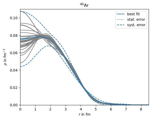
The package is currently in an development stage, and partly incomplete.
Use the package at your own risk and without any garanties.
This package was written by Frederic Noël.
I would like to thank my collaborators and office mates for meaningfull inputs. This website was build based on a template from github user charlyllo.
